In the field of fluid mechanics and hydraulics, the accurate determination of hydraulic coefficients is fundamental to the proper analysis and design of flow systems. While theoretical values for these coefficients can be estimated based on orifice geometry and flow conditions, experimental determination remains the most reliable method for obtaining accurate values for specific applications. The three primary hydraulic coefficients – coefficient of velocity (Cᵥ), coefficient of contraction (C꜀), and coefficient of discharge (C_d) – each represent different aspects of the flow behavior through an orifice and require distinct experimental approaches for their determination.
The importance of experimentally determining these coefficients cannot be overstated. Theoretical calculations, while useful for initial estimates, often fail to account for real-world factors such as surface roughness, edge conditions, approach flow conditions, and fluid properties. Experimental methods allow engineers to obtain coefficients that accurately reflect the specific conditions of their application, leading to more reliable system performance predictions and safer, more efficient designs.
Introduction to Hydraulic Coefficients
Hydraulic coefficients are dimensionless parameters that account for the various losses and deviations from ideal flow behavior in orifice flow. These coefficients are essential for converting theoretical flow equations into practical design tools that accurately predict real-world performance.
Coefficient of Velocity (Cᵥ)
The coefficient of velocity represents the ratio of the actual velocity at the vena contracta to the theoretical velocity predicted by Torricelli’s law. It accounts for losses due to friction and turbulence in the flow stream.
Where:
- V_actual is the actual velocity at the vena contracta
- V_theoretical is the velocity predicted by Torricelli’s equation
- g is the acceleration due to gravity
- H is the head of water above the orifice
Typical values of Cᵥ range from 0.95 to 0.99 for well-designed orifices, with the exact value depending on factors such as orifice shape, edge condition, and Reynolds number.
Coefficient of Contraction (C꜀)
The coefficient of contraction represents the ratio of the area of the jet at the vena contracta to the area of the orifice. It accounts for the contraction of the flow stream as it exits the orifice due to the inability of the fluid to make sharp turns at the orifice edges.
Where:
- A_jet is the area of the jet at the vena contracta
- A_orifice is the area of the orifice
Typical values of C꜀ range from 0.61 to 0.69 for sharp-edged orifices, with rounded orifices having higher values due to reduced contraction.
Coefficient of Discharge (C_d)
The coefficient of discharge represents the ratio of the actual discharge to the theoretical discharge. It combines the effects of both velocity and contraction losses.
Where:
- Q_actual is the measured actual discharge
- Q_theoretical is the theoretical discharge (A_orifice × √(2gH))
The coefficient of discharge is related to the other two coefficients by:
Typical values of C_d range from 0.58 to 0.65 for sharp-edged orifices, with variations based on orifice geometry and flow conditions.
Experimental Setup and Equipment
Proper experimental determination of hydraulic coefficients requires careful attention to the test setup and equipment selection. The accuracy of the results depends heavily on the quality of the experimental apparatus and the precision of the measurements.
Constant Head Tank
A constant head tank is essential for maintaining steady flow conditions during the experiment. This tank should be large enough to minimize fluctuations in water level during the test period and should be equipped with an overflow mechanism to maintain a constant head.
Key features of a constant head tank include:
- Large cross-sectional area to minimize head fluctuations
- Overflow weir to maintain constant water level
- Inlet supply system with flow control valve
- Transparent walls for visual observation of flow patterns
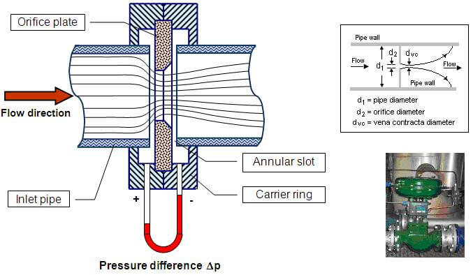
Orifice Plate
The orifice plate should be carefully machined to precise dimensions and installed perpendicular to the flow direction. The upstream face should be sharp and square-edged to promote proper flow contraction.
Specifications for the orifice plate include:
- Precise diameter measurement with calipers or micrometer
- Sharp, square upstream edge
- Smooth downstream edge
- Material resistant to corrosion and wear
Measuring Equipment
Several types of measuring equipment are required for the experimental determination of hydraulic coefficients:
- Calipers or micrometer: For precise measurement of orifice diameter and jet diameter at the vena contracta
- Measuring tank: For collecting and measuring the discharged water volume
- Stopwatch: For timing the collection period
- Pitot tube or trajectory board: For measuring the actual velocity of the jet
- Level gauges: For measuring water levels in the constant head tank
Measuring Tank
The measuring tank should be equipped with accurate volume measurement capabilities, typically through marked graduations or a weighing system. The tank should be large enough to collect a significant volume of water during the test period to minimize measurement errors.
Procedure for Coefficient of Velocity (Cᵥ)
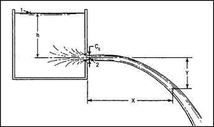
The coefficient of velocity can be determined using the trajectory method, which involves measuring the horizontal and vertical coordinates of the jet and using projectile motion equations to calculate the actual velocity.
Trajectory Method
The trajectory method is based on the principle that the jet exiting the orifice follows a parabolic path under the influence of gravity. By measuring the coordinates of points along this trajectory, the initial velocity can be determined.
Experimental Procedure
The procedure for determining Cᵥ using the trajectory method involves the following steps:
- Establish steady flow conditions in the constant head tank
- Measure and record the head of water above the orifice center (H)
- Set up a coordinate system with the origin at the vena contracta
- Mark several points along the jet trajectory at known horizontal distances (x)
- Measure the vertical distance (y) from the x-axis to the jet at each point
- Record multiple measurements to ensure accuracy
Analysis and Calculations
For projectile motion, the relationship between horizontal distance (x) and vertical distance (y) is given by:
Where:
- y is the vertical distance below the horizontal axis
- x is the horizontal distance from the origin
- g is the acceleration due to gravity
- V₀ is the initial velocity at the vena contracta
Rearranging to solve for V₀:
Using multiple (x,y) pairs, calculate V₀ for each pair and determine the average value. The theoretical velocity is:
Finally, the coefficient of velocity is:
Sources of Error and Accuracy Considerations
Several factors can affect the accuracy of the Cᵥ determination using the trajectory method:
- Air resistance: At high velocities, air resistance can affect the trajectory, leading to errors in velocity calculation
- Measurement precision: Errors in measuring x and y coordinates directly affect the calculated velocity
- Steady flow conditions: Fluctuations in head or flow rate can affect the trajectory shape
- Identification of vena contracta: Incorrect placement of the coordinate origin can introduce systematic errors
Procedure for Coefficient of Contraction (C꜀)
The coefficient of contraction is determined by measuring the diameter of the jet at the vena contracta and comparing it to the orifice diameter. This requires careful measurement techniques since the vena contracta is not always easily visible.
Measuring Jet Diameter at Vena Contracta
The vena contracta is the point of minimum cross-sectional area in the jet, located a short distance downstream of the orifice. Accurately locating and measuring this point is crucial for determining C꜀.
The location of the vena contracta depends on several factors:
- Orifice geometry and edge condition
- Reynolds number of the flow
- Approach flow conditions
For sharp-edged orifices, the vena contracta typically occurs at a distance of approximately 0.5 to 1.0 times the orifice diameter downstream of the orifice.
Experimental Procedure
The procedure for determining C꜀ involves the following steps:
- Establish steady flow conditions in the constant head tank
- Measure and record the orifice diameter using calipers or micrometer
- Identify the location of the vena contracta visually or using appropriate instruments
- Measure the jet diameter at the vena contracta using calipers positioned perpendicular to the jet
- Take multiple measurements at different angular positions around the jet circumference
- Record measurements and calculate average values
Analysis and Calculations
The coefficient of contraction is calculated as:
Where:
- d_jet is the diameter of the jet at the vena contracta
- d_orifice is the diameter of the orifice
It’s important to use the average of multiple diameter measurements to minimize measurement errors.
Alternative Methods
In cases where direct measurement of the jet diameter is difficult, alternative methods can be used:
- Tracer injection method: Injecting a colored tracer into the jet and photographing the contraction
- Laser sheet visualization: Using a laser sheet to illuminate the jet cross-section
- Pitot tube traverses: Measuring velocity profiles across the jet to identify the minimum area
Procedure for Coefficient of Discharge (C_d)
The coefficient of discharge can be determined directly by measuring the actual flow rate and comparing it to the theoretical flow rate. This is often the most straightforward of the three coefficients to determine experimentally.
Direct Measurement Method
The direct measurement method involves collecting the discharging water in a measuring tank for a specific time period and calculating the actual flow rate from the volume collected and the collection time.
Experimental Procedure
The procedure for determining C_d using the direct measurement method involves the following steps:
- Establish steady flow conditions in the constant head tank
- Measure and record the head of water above the orifice center (H)
- Measure and record the orifice diameter to calculate the orifice area (A_orifice)
- Position the measuring tank under the orifice discharge
- Start the collection process and simultaneously start the stopwatch
- Collect a known volume of water (or for a known time period)
- Stop the stopwatch when the collection is complete
- Record the volume collected and the time taken
- Repeat the measurement several times to ensure accuracy
Analysis and Calculations
The actual discharge is calculated as:
The theoretical discharge is:
Therefore, the coefficient of discharge is:
Accuracy Considerations
Several factors affect the accuracy of C_d determination:
- Volume measurement precision: The accuracy of the measuring tank graduations or weighing system
- Time measurement precision: The accuracy of the stopwatch or timing device
- Steady flow conditions: Maintaining constant head throughout the measurement period
- Orifice area measurement: Precise measurement of the orifice dimensions
Sample Experiment and Results
Let’s work through a complete example to illustrate the experimental determination of all three hydraulic coefficients:
Experimental Setup
Consider an experiment with the following parameters:
- Orifice diameter = 20 mm
- Head of water above orifice center (H) = 0.5 m
- Jet diameter at vena contracta = 16.8 mm
- Volume collected = 0.05 m³
- Time for collection = 72.5 seconds
- Trajectory measurements: At x = 0.3 m, y = 0.045 m
Determination of C꜀
Using the measured diameters:
Determination of C_d
First, calculate the actual discharge:
Calculate the orifice area:
Calculate the theoretical discharge:
Calculate the coefficient of discharge:
Determination of Cᵥ
Using the trajectory method with x = 0.3 m and y = 0.045 m:
Calculate the theoretical velocity:
Calculate the coefficient of velocity:
Verification of Relationship
Check if C_d = Cᵥ × C꜀:
The small difference (0.6%) is within experimental error and confirms the validity of the relationship between the three coefficients.
Error Analysis
Let’s examine the sensitivity of our results to potential measurement errors:
- Orifice diameter error of ±0.1 mm: This would change C꜀ by approximately ±1.0%
- Head measurement error of ±2 mm: This would change C_d by approximately ±0.4%
- Volume measurement error of ±0.5%: This would change C_d by ±0.5%
- Time measurement error of ±0.5 sec: This would change C_d by approximately ±0.7%
This analysis shows that time measurement accuracy is particularly important for C_d determination.
Applications in Engineering Practice
The experimental determination of hydraulic coefficients has numerous practical applications in engineering:
Hydraulic Structure Design
Engineers designing dams, spillways, and other hydraulic structures rely on accurate coefficient values to ensure proper performance:
- Sluice gate design for controlled discharge
- Spillway capacity calculations
- Outlet works sizing and performance prediction
Flow Measurement Systems
Many flow measurement devices depend on accurate coefficient values for proper calibration:
- Orifice meter calibration
- Weir and flume coefficient determination
- Venturi meter performance optimization
Industrial Process Optimization
In industrial applications, accurate coefficients help optimize process efficiency:
- Chemical processing vessel discharge rates
- Water treatment plant flow control
- Food and beverage processing line optimization
Advanced Experimental Techniques
Modern experimental techniques have enhanced the accuracy and capabilities of hydraulic coefficient determination:
Digital Imaging and PIV
Digital imaging techniques, including Particle Image Velocimetry (PIV), allow for detailed visualization and measurement of flow fields:
- High-resolution measurement of jet contraction
- Velocity field mapping around orifices
- Transient flow behavior analysis
Laser Doppler Anemometry
Laser Doppler Anemometry (LDA) provides precise point velocity measurements:
- Accurate velocity profile measurements
- Turbulence characterization
- Boundary layer analysis
Computational Fluid Dynamics Validation
Experimental results are increasingly used to validate computational models:
- CFD model calibration and verification
- Turbulence model validation
- Scale effect investigation
Quality Control and Standards
Various standards and guidelines exist for the experimental determination of hydraulic coefficients:
International Standards
Organizations such as ISO and ASTM have published standards for hydraulic coefficient determination:
- ISO 5167 for flow measurement using pressure differential devices
- ASTM D5616 for measuring hydraulic conductivity of soils
Best Practices
Following established best practices ensures reliable results:
- Proper calibration of all measuring instruments
- Adequate sampling periods for statistical validity
- Control of environmental conditions (temperature, pressure)
- Documentation of all experimental conditions and procedures
Conclusion
The experimental determination of hydraulic coefficients is a fundamental aspect of hydraulic engineering that provides the foundation for accurate flow analysis and system design. By understanding and properly applying the procedures for determining the coefficient of velocity, coefficient of contraction, and coefficient of discharge, engineers can ensure that their designs accurately reflect real-world performance.
The sample experiment demonstrates how all three coefficients can be determined in a single test setup, and the verification of the relationship C_d = Cᵥ × C꜀ provides a check on the consistency of the measurements. The error analysis shows which measurements are most critical for accuracy, helping experimenters focus their efforts on the most important aspects of the procedure.
The wide range of applications, from dam design to industrial process optimization, underscores the importance of accurate coefficient determination in engineering practice. The continuing development of advanced experimental techniques, including digital imaging and computational validation, promises even greater accuracy and understanding of hydraulic phenomena in the future.
As engineering systems become more complex and performance requirements more stringent, the fundamental principles of experimental coefficient determination remain essential tools for analysis and design. Modern computational methods and measurement techniques continue to enhance our understanding and application of these principles, enabling more efficient and reliable hydraulic systems.
Future developments in sensor technology, data acquisition systems, and computational modeling will likely provide even more accurate methods for determining hydraulic coefficients, further expanding their utility in engineering applications. The continued importance of experimental validation ensures that these fundamental principles will remain relevant for generations of engineers to come.
Engineers should always remember that while theoretical calculations provide valuable initial estimates, experimental determination remains the gold standard for obtaining accurate coefficients for specific applications. Proper experimental technique, careful measurement, and thorough analysis are essential for reliable results that can be confidently applied to engineering design and analysis.