In the study of fluid mechanics and hydraulics, understanding the behavior of fluids flowing through orifices is fundamental to numerous engineering applications. Central to this understanding are the three key hydraulic coefficients: coefficient of velocity (Cᵥ), coefficient of contraction (C꜀), and coefficient of discharge (C_d). While each of these coefficients represents a distinct aspect of the flow behavior, they are not independent of one another. A fundamental relationship exists between them that is both mathematically elegant and practically significant.
This relationship, expressed as C_d = Cᵥ × C꜀, forms a cornerstone of orifice flow analysis and has profound implications for both theoretical understanding and practical application. By exploring this relationship in detail, we gain deeper insights into the nature of fluid flow through orifices and develop more robust methods for analyzing and designing hydraulic systems.
Introduction to Hydraulic Coefficients
Before delving into the relationship between the hydraulic coefficients, it’s essential to clearly understand what each coefficient represents and how it contributes to our overall understanding of orifice flow.
Coefficient of Velocity (Cᵥ)
The coefficient of velocity quantifies the efficiency of the energy conversion process in orifice flow. It represents the ratio of the actual velocity at the vena contracta to the theoretical velocity predicted by Torricelli’s law.
Where:
- V_actual is the actual velocity at the vena contracta
- V_theoretical is the theoretical velocity from Torricelli’s equation (√(2gH))
- g is the acceleration due to gravity
- H is the head of water above the orifice center
The coefficient of velocity accounts for losses due to friction, turbulence, and other dissipative effects that reduce the actual velocity below the theoretical value. For well-designed orifices, Cᵥ typically ranges from 0.95 to 0.99, indicating that most of the theoretical velocity is achieved in practice.
Coefficient of Contraction (C꜀)
The coefficient of contraction addresses the geometric aspect of orifice flow by quantifying the reduction in flow area as the fluid exits the orifice. It represents the ratio of the area of the jet at the vena contracta to the area of the orifice itself.
Where:
- A_jet is the cross-sectional area of the jet at the vena contracta
- A_orifice is the cross-sectional area of the orifice
The coefficient of contraction arises because fluids cannot make sharp turns at solid boundaries. As fluid approaches the orifice edges, it curves inward, resulting in a jet with a smaller cross-sectional area than the orifice. For sharp-edged orifices, C꜀ typically ranges from 0.61 to 0.69, reflecting the significant contraction that occurs.
Coefficient of Discharge (C_d)
The coefficient of discharge combines both the velocity and contraction effects to provide an overall measure of orifice efficiency. It represents the ratio of the actual discharge to the theoretical discharge.
Where:
- Q_actual is the measured actual discharge through the orifice
- Q_theoretical is the theoretical discharge (A_orifice × √(2gH))
The coefficient of discharge is the most commonly used coefficient in practical applications because it directly relates to the quantity of practical interest – the actual flow rate. For sharp-edged orifices, C_d typically ranges from 0.58 to 0.65, representing the combined effect of velocity and contraction losses.
Fundamental Definitions and Concepts
To properly understand the relationship between the hydraulic coefficients, we need to establish precise definitions and explore the underlying physical concepts.
Definition of Cᵥ
The coefficient of velocity is fundamentally a measure of how effectively the potential energy of the fluid is converted to kinetic energy. In an ideal, frictionless system, all potential energy would be converted to kinetic energy, resulting in Cᵥ = 1.0. In real systems, some energy is lost to friction and turbulence, reducing the actual velocity and resulting in Cᵥ < 1.0.
The actual velocity at the vena contracta can be expressed as:
Definition of C꜀
The coefficient of contraction reflects the geometric constraints imposed by the fluid’s inability to follow sharp corners. This phenomenon is a direct consequence of the no-slip condition at solid boundaries and the continuity of the fluid.
The area of the jet at the vena contracta can be expressed as:
Definition of C_d
The coefficient of discharge represents the overall efficiency of the orifice as a flow control device. It combines both the energetic and geometric aspects of the flow to provide a single, practical measure of performance.
The actual discharge through the orifice can be expressed as:
Derivation of the Relationship
The relationship between the three hydraulic coefficients can be derived by examining the definition of actual discharge in terms of the velocity and area at the vena contracta.
Starting with the Definition of Actual Discharge
The actual discharge through an orifice is the product of the actual velocity at the vena contracta and the actual area of the jet at that point:
Substituting the Definitions of the Coefficients
We can substitute the expressions for V_actual and A_jet in terms of the hydraulic coefficients:
Substituting these into the discharge equation:
Relating to the Coefficient of Discharge
We also know that:
Setting the two expressions for Q_actual equal to each other:
Dividing both sides by (A_orifice × √(2gH)):
This derivation shows that the relationship C_d = Cᵥ × C꜀ follows directly from the definitions of the three coefficients and the fundamental principle that discharge equals velocity times area.
Physical Interpretation of the Relationship
The relationship C_d = Cᵥ × C꜀ has a clear physical interpretation:
- Cᵥ accounts for the efficiency of energy conversion (how fast the fluid moves)
- C꜀ accounts for the geometric efficiency (how much area is available for flow)
- C_d represents the combined efficiency of both processes
This multiplicative relationship makes intuitive sense because both factors must be considered to determine the overall flow rate. If either the velocity efficiency or the area efficiency is reduced, the overall discharge efficiency will be reduced proportionally.
Verification Through Example Calculations
Let’s examine the relationship through a practical example to verify its validity and explore its implications.
Sample Problem
Consider an experiment with a sharp-edged orifice under the following conditions:
- Orifice diameter = 25 mm
- Head of water = 0.6 m
- Jet diameter at vena contracta = 21.2 mm
- Actual velocity at vena contracta = 3.35 m/s
- Actual discharge = 0.00118 m³/s
Calculation of Cᵥ
First, calculate the theoretical velocity:
Then calculate Cᵥ:
Calculation of C꜀
Calculate the areas:
Then calculate C꜀:
Calculation of C_d
Calculate the theoretical discharge:
Then calculate C_d:
Verification of the Relationship
Check if C_d = Cᵥ × C꜀:
The difference of 0.3% is within experimental error and confirms the validity of the relationship. This close agreement demonstrates that the fundamental relationship holds true for real-world conditions.
Implications of the Relationship
The verification of the relationship has several important implications:
- If any two coefficients are known, the third can be calculated
- The relationship provides a check on experimental measurements
- It demonstrates the consistency of the theoretical framework
Practical Applications of the Relationship
The relationship C_d = Cᵥ × C꜀ has numerous practical applications in engineering practice, from design calculations to experimental validation.
Design Calculations
In hydraulic system design, engineers often need to determine orifice sizes for specific flow requirements. The relationship allows them to work with whichever coefficients are most readily available:
- If C_d values are available from standard tables, they can be used directly
- If separate Cᵥ and C꜀ values are available, they can be multiplied to obtain C_d
- If only one coefficient is known, the relationship can be used with typical values for the other
Experimental Validation
In experimental work, the relationship provides a valuable check on measurement accuracy:
- If all three coefficients are measured independently, their relationship should hold
- Discrepancies may indicate measurement errors or unaccounted-for effects
- The relationship can be used to estimate one coefficient if the other two are measured
System Optimization
Understanding the relationship helps engineers optimize hydraulic systems by identifying which aspects of performance to target for improvement:
- If C_d is low due to low Cᵥ, focus on reducing friction and turbulence
- If C_d is low due to low C꜀, focus on orifice geometry and edge design
- The relationship shows that improvements in either coefficient will proportionally improve overall performance
Factors Affecting the Coefficients
Understanding how various factors affect the individual coefficients helps explain variations in their relationship and provides insights for system optimization.
Orifice Geometry
The shape and edge condition of the orifice significantly affect both C꜀ and Cᵥ:
- Sharp-edged orifices: Produce significant contraction (low C꜀) but relatively high velocity efficiency (high Cᵥ)
- Rounded orifices: Reduce contraction (higher C꜀) but may reduce velocity efficiency (lower Cᵥ)
- Beveled edges: Can optimize the balance between C꜀ and Cᵥ for specific applications
Reynolds Number Effects
The Reynolds number, which characterizes the flow regime, affects all three coefficients:
Where:
- V is the velocity
- D is a characteristic length (orifice diameter)
- ν is the kinematic viscosity
At low Reynolds numbers (laminar flow), all coefficients may vary significantly with flow rate. At high Reynolds numbers (turbulent flow), the coefficients tend to stabilize at relatively constant values.
Approach Conditions
The conditions in the approach channel affect the coefficients:
- Approach velocity: High approach velocities can affect the effective head and velocity distribution
- Turbulence in approach flow: Can affect the flow pattern at the orifice
- Boundary layer development: Can influence the contraction and velocity profiles
Advanced Considerations
For specialized applications or high-precision requirements, engineers may need to consider additional factors that affect the relationship between hydraulic coefficients.
Unsteady Flow Effects
In unsteady flow conditions, the relationship may be affected by:
- Time-dependent changes in the vena contracta location
- Dynamic effects on velocity profiles
- Inertia effects that may temporarily alter the coefficient values
Compressibility Effects
For high-velocity gas flows where compressibility becomes significant:
- The basic relationship still holds but with modified definitions
- Additional coefficients may be needed to account for compressibility effects
- The relationship becomes more complex due to density variations
Non-Newtonian Fluids
For non-Newtonian fluids with variable viscosity:
- The coefficients may vary with shear rate
- The relationship may need modification for specific fluid models
- Time-dependent effects may be significant for thixotropic or rheopectic fluids
Measurement and Experimental Determination
Understanding how each coefficient is measured helps appreciate the practical significance of their relationship.
Coefficient of Velocity (Cᵥ)
Cᵥ is typically determined using:
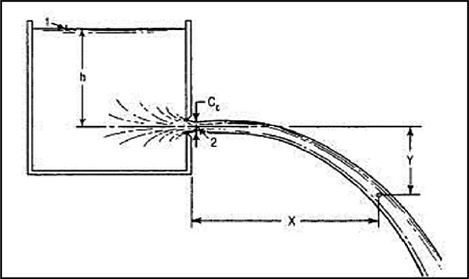
- Trajectory method: Measuring jet coordinates and using projectile motion equations
- Pitot tube measurements: Direct velocity measurement at the vena contracta
- Laser Doppler anemometry: High-precision velocity measurements
Coefficient of Contraction (C꜀)
C꜀ is typically determined using:
- Direct measurement: Calipers or micrometers to measure jet diameter
- Tracer injection: Visualizing the contraction with colored fluid
- PIV (Particle Image Velocimetry): Mapping flow fields to identify vena contracta
Coefficient of Discharge (C_d)
C_d is typically determined using:
- Direct measurement: Weighing or volumetric collection of discharged fluid
- Flow meters: Using calibrated flow measurement devices
- Weirs and flumes: For open channel flow applications
Comparison with Other Flow Devices
Understanding how the relationship applies to other flow measurement devices provides broader context:
| Flow Device | C_d Relationship | Typical C_d Values | Comments |
|---|---|---|---|
| Sharp-edged orifice | C_d = Cᵥ × C꜀ | 0.58-0.65 | Classic application of the relationship |
| Venturi meter | C_d ≈ Cᵥ (C꜀ ≈ 1) | 0.95-0.98 | Minimal contraction due to gradual transition |
| Nozzle meter | C_d ≈ Cᵥ (C꜀ ≈ 1) | 0.95-0.99 | Streamlined design minimizes contraction |
| Weirs | More complex relationship | 0.60-0.70 | Depends on weir geometry and approach conditions |
This comparison shows that while the fundamental relationship C_d = Cᵥ × C꜀ applies to orifice flow, other devices may have different relationships due to their specific geometries and flow characteristics.
Conclusion
The relationship between hydraulic coefficients, expressed as C_d = Cᵥ × C꜀, represents a fundamental principle in fluid mechanics that elegantly connects the energetic and geometric aspects of orifice flow. This relationship is not merely a mathematical convenience but reflects deep physical principles about how fluids behave when flowing through restrictions.
The derivation of this relationship from first principles demonstrates its theoretical soundness, while the verification through example calculations confirms its practical validity. The close agreement between calculated and measured values in real-world applications underscores the robustness of the underlying theory.
The practical applications of this relationship are extensive and significant. Engineers can use it to:
- Simplify design calculations by working with whichever coefficients are most readily available
- Validate experimental measurements and identify potential sources of error
- Optimize system performance by understanding which aspects of flow behavior to target for improvement
Understanding how various factors affect the individual coefficients provides valuable insights for system design and optimization. The relationship shows that improvements in either velocity efficiency or area efficiency will proportionally improve overall discharge efficiency, guiding engineers toward the most effective optimization strategies.
As engineering systems become more sophisticated and performance requirements more demanding, the fundamental relationship between hydraulic coefficients remains a cornerstone of hydraulic engineering practice. Modern computational methods and measurement techniques continue to enhance our understanding and application of these principles, enabling more efficient and reliable hydraulic systems.
Future developments in fluid dynamics, materials science, and measurement technology will likely provide even more refined methods for determining and applying hydraulic coefficients, but the fundamental relationship C_d = Cᵥ × C꜀ will remain unchanged. This enduring principle testifies to the power of fundamental physical laws in describing and predicting complex engineering phenomena.
Engineers should always remember that while this relationship is mathematically exact, its practical application requires careful consideration of the specific conditions and limitations of each situation. Proper understanding of the underlying assumptions and their validity for specific applications is essential for reliable engineering practice.
The relationship between hydraulic coefficients exemplifies the elegance and power of engineering science – simple in form but profound in implication, providing both practical tools for design and deeper insights into the nature of fluid behavior.