In the field of fluid mechanics, understanding the behavior of fluids under various conditions is crucial for engineers. One of the fundamental problems in this domain is calculating the time it takes for a fluid to empty from a tank through an orifice. This seemingly simple problem has significant practical applications in various engineering systems, from water reservoirs to industrial storage tanks. The calculation involves understanding fluid dynamics principles and applying mathematical models to predict the behavior of the fluid over time.
The problem of calculating the time required for a fluid level in a tank to drop from an initial height to a final height is not only academically interesting but also practically important. Engineers need to determine this time for various applications such as designing emergency drainage systems, sizing storage tanks, and optimizing industrial processes. The solution to this problem involves applying fundamental principles of fluid mechanics and calculus.
Theoretical Principles
The foundation of our analysis lies in Torricelli’s Law, which describes the velocity of efflux from an orifice. This law, named after the Italian physicist Evangelista Torricelli, states that the speed of efflux of a fluid under the force of gravity through an orifice is proportional to the square root of the height of fluid above the opening. This principle is fundamental to understanding fluid flow from tanks and vessels.
Torricelli’s Law can be mathematically expressed as:
Where:
- v is the velocity of the fluid at the orifice
- g is the acceleration due to gravity (approximately 9.81 m/s²)
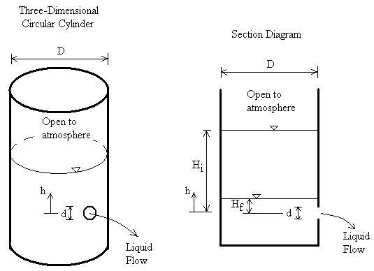
- h is the height of the fluid above the orifice
This equation shows that the velocity of the fluid increases with the square root of the height of the fluid column. As the tank empties and the fluid level drops, the velocity of the fluid exiting through the orifice also decreases. This relationship is crucial for understanding how the emptying process evolves over time.
It’s important to note that Torricelli’s Law is based on several assumptions:
- The fluid is incompressible
- The flow is steady and frictionless
- The orifice is small compared to the tank dimensions
- The velocity of the fluid at the surface is negligible compared to the velocity at the orifice
While these assumptions simplify the analysis, they also limit the accuracy of the model in certain real-world situations. However, for many engineering applications, Torricelli’s Law provides a good approximation that is both mathematically tractable and practically useful.
Derivation for a Uniform Cross-Section Tank
For a tank with a uniform cross-sectional area, the derivation of the time required to empty the tank is relatively straightforward. Let’s consider a cylindrical tank with a constant cross-sectional area A_tank and an orifice at the bottom with area A_orifice.
To derive the equation, we need to establish a relationship between the change in volume in the tank and the discharge rate through the orifice. This requires setting up a differential equation that describes the system’s behavior.
The rate of change of volume in the tank is equal to the negative of the discharge rate through the orifice:
Where:
- A_tank is the cross-sectional area of the tank
- dh is the change in fluid height
- C_d is the coefficient of discharge
- A_orifice is the area of the orifice
- g is the acceleration due to gravity
- h is the height of the fluid
- dt is the change in time
The coefficient of discharge (C_d) accounts for the losses due to friction and the contraction of the jet at the vena contracta. Its value typically ranges from 0.6 to 0.9 depending on the shape and condition of the orifice.
To solve this differential equation, we rearrange terms to separate the variables:
Integrating both sides of the equation between the initial height H₁ and final height H₂ gives us the total time T required to empty the tank from H₁ to H₂:
Performing the integration:
Simplifying this expression:
This equation provides the time required to lower the fluid level in a tank with uniform cross-section from an initial height H₁ to a final height H₂. It’s worth noting that if we want to completely empty the tank, we set H₂ = 0, which simplifies the equation to:
This derivation assumes that the tank has a constant cross-sectional area throughout its height. For tanks with varying cross-sectional areas, such as conical or spherical tanks, the derivation becomes more complex and requires modification of the approach.
Derivation for Variable Cross-Section (e.g., Hemispherical Tank)
For tanks with variable cross-sectional areas, the derivation becomes more complex because the area of the tank A_tank is now a function of height h. Let’s consider a hemispherical tank as an example, where the cross-sectional area changes with the height of the fluid.
For a hemispherical tank of radius R, the cross-sectional area at any height h can be determined using geometry. At height h from the bottom of the hemisphere, the cross-sectional area is:
The differential equation now becomes:
Rearranging to separate variables:
Integrating both sides:
This integral is more complex to solve than in the uniform cross-section case. The integration involves terms with fractional powers of h, which require more advanced mathematical techniques to solve. The result will be a more complex expression for the time T, which depends on the specific geometry of the tank.
For other tank geometries, such as conical tanks or tanks with complex shapes, similar approaches are used. The key is to express the cross-sectional area A_tank as a function of height h and then integrate the resulting differential equation. In some cases, numerical methods may be required to obtain a solution.
Sample Problem
Let’s work through a sample problem to illustrate the application of these principles. Consider a cylindrical water tank with a diameter of 2 meters and a height of 3 meters. The tank is initially filled with water to a height of 2.5 meters. There is a circular orifice at the bottom of the tank with a diameter of 5 cm. The coefficient of discharge for the orifice is 0.62. We want to calculate the time required to empty the tank completely.
First, let’s determine the necessary parameters:
- Tank diameter = 2 m, so radius = 1 m
- Tank cross-sectional area A_tank = π × (1)² = π m²
- Initial height H₁ = 2.5 m
- Final height H₂ = 0 m (completely empty)
- Orifice diameter = 5 cm = 0.05 m, so radius = 0.025 m
- Orifice area A_orifice = π × (0.025)² = 0.00196 m²
- Coefficient of discharge C_d = 0.62
- Acceleration due to gravity g = 9.81 m/s²
Using our derived formula for a uniform cross-section tank:
Substituting the values:
Calculating step by step:
Converting to minutes:
Therefore, it would take approximately 30.7 minutes to completely empty the tank under the given conditions.
This calculation assumes ideal conditions and does not account for factors such as:
- Viscosity of the fluid
- Surface tension effects
- Air resistance and turbulence
- Changes in the coefficient of discharge at different flow rates
- Imperfections in the orifice shape
In real-world applications, engineers often apply safety factors to account for these uncertainties and ensure that their designs are conservative enough to handle variations in actual conditions.
Factors Affecting the Emptying Time
Several factors influence the time required to empty a tank through an orifice. Understanding these factors is crucial for engineers when designing systems that involve fluid discharge through orifices.
Tank Geometry
The shape and size of the tank significantly affect the emptying time. Tanks with larger cross-sectional areas take longer to empty because there is more fluid to discharge. The variation in cross-sectional area with height also affects the emptying profile. In tanks with uniform cross-sections, the discharge rate decreases linearly with the square root of the height. In tanks with varying cross-sections, the relationship is more complex.
Orifice Size and Shape
The size and shape of the orifice directly impact the discharge rate. Larger orifices allow more fluid to flow through in a given time, reducing the emptying time. The shape of the orifice also affects the coefficient of discharge, with sharp-edged orifices typically having lower coefficients than well-rounded orifices.
Fluid Properties
The properties of the fluid being discharged also play a role. While our derivation assumes incompressible fluids, real fluids may exhibit compressibility effects at high velocities. Viscosity affects the flow characteristics, particularly for small orifices or highly viscous fluids. Surface tension can also influence the flow, especially for very small orifices.
Coefficient of Discharge
The coefficient of discharge accounts for losses in the system. These losses include friction losses, contraction losses at the vena contracta, and other minor losses. The value of C_d depends on the orifice geometry, Reynolds number of the flow, and surface roughness.
Initial Fluid Height
As evident from our equations, the initial height of the fluid has a significant impact on the emptying time. Since the time is proportional to the square root of the initial height, doubling the initial height increases the emptying time by approximately 41% (√2 ≈ 1.41).
Applications in Engineering
The concept of time required to empty a tank through an orifice has numerous practical applications in various engineering disciplines:
Water Supply Systems
In water supply systems, understanding the emptying time of storage tanks is crucial for system design and management. Engineers use these calculations to determine the capacity of tanks needed to meet demand during peak periods and to plan for emergency situations where water supply might be interrupted.
Industrial Processes
Many industrial processes involve the controlled discharge of liquids from tanks. For example, in chemical processing plants, reaction vessels need to be emptied at controlled rates to ensure proper mixing and reaction times. In food processing, tanks containing liquids must be emptied efficiently while maintaining product quality.
Flood Control and Drainage
Engineers designing flood control systems and drainage networks use these principles to calculate the time required for water to drain from retention basins, culverts, and other structures. This information is crucial for sizing these structures appropriately to handle expected flood volumes.
Hydraulic Machinery
The design of hydraulic machinery, such as hydraulic presses and accumulators, relies on understanding fluid discharge characteristics. Engineers use these calculations to determine the performance characteristics of these devices and to optimize their operation.
Advanced Considerations
While our basic derivation provides a good foundation for understanding the emptying process, several advanced considerations can affect the accuracy of predictions in real-world applications:
Unsteady Flow Effects
Our derivation assumes steady flow conditions, but in reality, the flow is unsteady as the fluid level changes. This can lead to slight deviations from the predicted emptying time, particularly for tanks with rapidly changing cross-sectional areas.
Compressibility Effects
For very high-velocity flows or when dealing with gases, compressibility effects become significant. The density of the fluid changes with pressure, which affects the flow rate and, consequently, the emptying time.
Viscous Effects
For highly viscous fluids or flows through very small orifices, viscous effects become dominant. The flow may transition from turbulent to laminar, which significantly changes the relationship between pressure and flow rate.
Surface Tension Effects
For very small orifices or low-density fluids, surface tension effects can influence the flow. These effects can cause the formation of droplets rather than a continuous jet, which affects the discharge rate.
Temperature Effects
Temperature changes can affect fluid properties such as viscosity and density, which in turn affect the flow characteristics. In applications where temperature variations are significant, these effects must be considered in the calculations.
Numerical Methods for Complex Geometries
For tanks with complex geometries where analytical solutions are difficult or impossible to obtain, numerical methods can be employed. These methods involve discretizing the differential equations and solving them using computational techniques.
Finite difference methods can be used to approximate the derivatives in the differential equations, allowing for step-by-step calculation of the fluid height and emptying time. More advanced techniques, such as finite element methods or computational fluid dynamics (CFD), can provide detailed insights into the flow patterns and pressure distributions within the tank.
Conclusion
The calculation of time required to empty a tank through an orifice is a fundamental problem in fluid mechanics with wide-ranging applications in engineering. By applying Torricelli’s Law and setting up appropriate differential equations, we can derive formulas for predicting the emptying time for various tank geometries.
For tanks with uniform cross-sections, the derivation is relatively straightforward and results in a simple formula that engineers can use for quick calculations. For tanks with variable cross-sections, the mathematics becomes more complex, but the underlying principles remain the same.
The practical applications of this knowledge span numerous engineering disciplines, from water supply systems to industrial process design. Understanding the factors that affect emptying time allows engineers to optimize their designs for efficiency and safety.
While our basic derivations provide good approximations for many applications, engineers must be aware of the limitations of these models and consider advanced factors such as unsteady flow effects, compressibility, viscosity, and surface tension when dealing with more complex or critical applications.
Modern computational tools have made it possible to analyze complex geometries and flow conditions that would be difficult or impossible to solve analytically. However, the fundamental principles discussed here remain the foundation upon which these advanced analyses are built.
As with all engineering calculations, it’s important to validate theoretical predictions with experimental data whenever possible and to apply appropriate safety factors to account for uncertainties in real-world conditions.