In the field of thermal engineering and power generation, numerous thermodynamic cycles have been developed to convert heat energy into mechanical work. Among these, the Ericsson cycle stands out as an ideal thermodynamic cycle that uses external heat exchange, similar to the Stirling cycle. Named after John Ericsson, a Swedish-American inventor who developed it in the 19th century, this cycle represents an important theoretical framework for understanding heat engine performance and efficiency limits.
The Ericsson cycle is particularly notable because its theoretical efficiency equals that of the Carnot cycle, the maximum possible efficiency for any heat engine operating between two temperature reservoirs. This makes it an important subject of study in thermodynamics, even though practical implementation has faced significant challenges that have limited its widespread use in commercial applications.
Introduction to the Ericsson Cycle
The Ericsson cycle is a thermodynamic cycle that describes the operation of a theoretical heat engine using external heat exchange. It consists of four distinct processes that form a closed loop on thermodynamic diagrams, returning the working fluid to its initial state after completing one cycle.
The cycle is characterized by two isothermal processes (constant temperature) and two isobaric processes (constant pressure), making it distinct from other common cycles like the Otto cycle (isochoric processes) or the Diesel cycle (isochoric and isentropic processes). This unique combination of processes gives the Ericsson cycle its distinctive properties and theoretical advantages.
John Ericsson, the cycle’s namesake, was a prolific inventor who also developed the screw propeller and contributed to the design of the USS Monitor, an ironclad warship used during the American Civil War. His work on the Ericsson cycle was part of his broader efforts to improve the efficiency of heat engines in the mid-19th century.
The Four Processes of the Ericsson Cycle
The Ericsson cycle consists of four distinct thermodynamic processes that together form a complete cycle. Understanding each process is crucial for analyzing the cycle’s performance and characteristics.
Process 1-2: Isothermal Compression (Heat Rejection)
The cycle begins with isothermal compression, where the working fluid is compressed while maintaining a constant low temperature (T_L). During this process:
- Temperature remains constant at T_L
- Pressure increases as volume decreases
- Heat is rejected to the cold reservoir
- Work is done on the working fluid
This process is similar to the isothermal compression in the Carnot cycle and represents the “waste heat” rejection portion of the cycle.
Process 2-3: Isobaric Heating (Constant Pressure Heat Addition)
Following the isothermal compression, the working fluid undergoes isobaric heating, typically with a regenerator:
- Pressure remains constant
- Temperature increases from T_L to T_H
- Volume increases as temperature rises
- Heat is added from an external source or regenerator
This process distinguishes the Ericsson cycle from the Carnot cycle, which uses isentropic processes for heating and cooling. The use of isobaric processes allows for different heat transfer characteristics.
Process 3-4: Isothermal Expansion (Heat Addition)
The third process is isothermal expansion, where the working fluid expands while maintaining a constant high temperature (T_H):
- Temperature remains constant at T_H
- Pressure decreases as volume increases
- Heat is added from the hot reservoir
- Work is done by the working fluid
This is the power stroke of the cycle, where the majority of the useful work is produced. It’s analogous to the isothermal expansion in the Carnot cycle.
Process 4-1: Isobaric Cooling (Constant Pressure Heat Rejection)
The cycle completes with isobaric cooling, often involving a regenerator:
- Pressure remains constant
- Temperature decreases from T_H to T_L
- Volume decreases as temperature drops
- Heat is rejected to the cold reservoir or stored in regenerator
This final process returns the working fluid to its initial state, completing the cycle and preparing it for the next iteration.
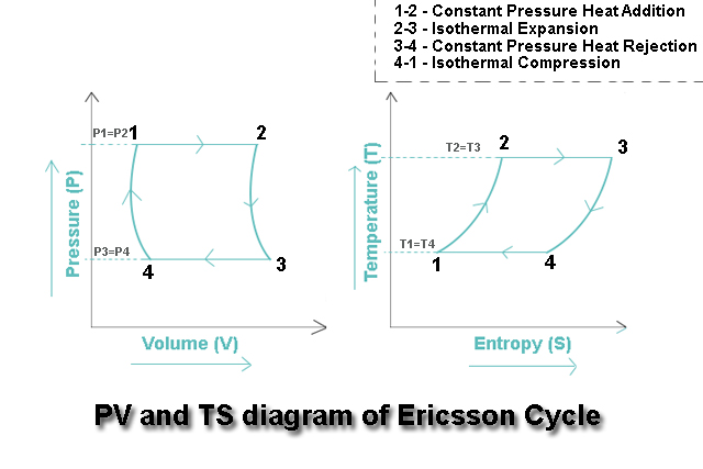
P-V (Pressure-Volume) Diagram
The Pressure-Volume (P-V) diagram is one of the most直观 ways to visualize the Ericsson cycle and understand the work interactions during each process. This diagram plots pressure on the vertical axis and specific volume on the horizontal axis.
Characteristics of the P-V Diagram
The P-V diagram for the Ericsson cycle has several distinctive characteristics:
- Two Horizontal Lines: Represent the isobaric processes (constant pressure) – Process 2-3 and Process 4-1
- Two Curved Lines: Represent the isothermal processes – Process 1-2 (isothermal compression) and Process 3-4 (isothermal expansion)
- Rectangular Appearance: The combination of horizontal and curved lines gives the cycle a somewhat rectangular shape, though with curved sides
- Work Representation: The area enclosed by the cycle represents the net work output per cycle
Process Representation on P-V Diagram
Each process is represented distinctly on the P-V diagram:
- Process 1-2 (Isothermal Compression): A curve moving from lower right to upper left, showing decreasing volume and increasing pressure at constant temperature T_L
- Process 2-3 (Isobaric Heating): A horizontal line moving from left to right, showing increasing volume at constant pressure P_H
- Process 3-4 (Isothermal Expansion): A curve moving from upper left to lower right, showing increasing volume and decreasing pressure at constant temperature T_H
- Process 4-1 (Isobaric Cooling): A horizontal line moving from right to left, showing decreasing volume at constant pressure P_L
Work Calculations from P-V Diagram
The work done during each process can be determined from the P-V diagram:
- Isothermal Processes: Work is calculated using W = nRT ln(V₂/V₁)
- Isobaric Processes: Work is calculated using W = P(V₂ – V₁)
- Net Work: The difference between work output (Process 3-4) and work input (Process 1-2), represented by the enclosed area
T-S (Temperature-Entropy) Diagram
The Temperature-Entropy (T-S) diagram provides another perspective on the Ericsson cycle, emphasizing the heat transfer characteristics and entropy changes during each process. This diagram plots temperature on the vertical axis and specific entropy on the horizontal axis.
Characteristics of the T-S Diagram
The T-S diagram for the Ericsson cycle has distinct characteristics that make it particularly useful for analyzing heat transfer:
- Two Vertical Lines: Represent the isothermal processes (constant temperature) – Process 1-2 and Process 3-4
- Two Horizontal Lines: Represent the isobaric processes – Process 2-3 and Process 4-1
- Rectangular Shape: With perfect regeneration, the cycle forms an exact rectangle on the T-S diagram
- Heat Transfer Representation: The area under each process line represents the heat transfer during that process
Process Representation on T-S Diagram
Each process has a distinctive representation on the T-S diagram:
- Process 1-2 (Isothermal Compression): A vertical line moving downward, showing decreasing entropy at constant temperature T_L
- Process 2-3 (Isobaric Heating): A horizontal line moving to the right, showing increasing entropy at increasing temperature
- Process 3-4 (Isothermal Expansion): A vertical line moving upward, showing increasing entropy at constant temperature T_H
- Process 4-1 (Isobaric Cooling): A horizontal line moving to the left, showing decreasing entropy at decreasing temperature
Heat Transfer Calculations from T-S Diagram
The heat transfer during each process can be determined from the T-S diagram:
- Isothermal Processes: Heat transfer is calculated using Q = TΔS
- Isobaric Processes: Heat transfer requires integration or use of specific heat relationships
- Net Heat Input: The difference between heat added (Processes 3-4 and 2-3) and heat rejected (Processes 1-2 and 4-1)
Efficiency Analysis
One of the most remarkable characteristics of the Ericsson cycle is its theoretical efficiency, which equals that of the Carnot cycle when operating between the same temperature limits.
Theoretical Efficiency
The thermal efficiency of the Ericsson cycle is given by:
Where:
- η is the thermal efficiency
- T_L is the absolute temperature of the cold reservoir
- T_H is the absolute temperature of the hot reservoir
This is identical to the Carnot efficiency, making the Ericsson cycle theoretically as efficient as possible for any heat engine operating between the same temperature limits.
Comparison with Other Cycles
Comparing the Ericsson cycle with other thermodynamic cycles:
| Cycle | Processes | Theoretical Efficiency | Comments |
|---|---|---|---|
| Carnot | 2 Isothermal, 2 Isentropic | η = 1 – (T_L / T_H) | Maximum possible efficiency |
| Ericsson | 2 Isothermal, 2 Isobaric | η = 1 – (T_L / T_H) | Equals Carnot efficiency |
| Stirling | 2 Isothermal, 2 Isochoric | η = 1 – (T_L / T_H) | Equals Carnot efficiency |
| Rankine | 2 Isobaric, 2 Isentropic | Less than Carnot | Practical steam cycle |
| Brayton | 2 Isobaric, 2 Isentropic | Less than Carnot | Gas turbine cycle |
Factors Affecting Practical Efficiency
While the theoretical efficiency matches the Carnot efficiency, practical implementations face several challenges:
- Regenerator Effectiveness: Imperfect heat exchange in regenerators reduces efficiency
- Pressure Drops: Friction losses in heat exchangers and piping
- Heat Transfer Limitations: Finite heat transfer rates affect cycle performance
- Working Fluid Properties: Real gas behavior deviates from ideal assumptions
Regeneration in the Ericsson Cycle
Regeneration is a key feature of the Ericsson cycle that distinguishes it from the Carnot cycle and contributes to its high theoretical efficiency. A regenerator is a heat exchanger that stores heat from the hot portion of the cycle and releases it during the cold portion.
Principle of Regeneration
The regenerator operates on the principle of thermal energy storage and recovery:
- During Process 4-1 (isobaric cooling), heat is transferred to the regenerator material
- During Process 2-3 (isobaric heating), heat is transferred from the regenerator material to the working fluid
- This internal heat transfer reduces the external heat input required
- In an ideal regenerator, the heat stored equals the heat recovered
Benefits of Regeneration
Regeneration provides several advantages in the Ericsson cycle:
- Improved Efficiency: Reduces the amount of external heat required
- Reduced Heat Rejection: Less heat needs to be rejected to the cold reservoir
- Temperature Matching: Allows better matching of heat source and sink temperatures
- Economic Benefits: Reduces fuel consumption and operating costs
Regenerator Design Considerations
Effective regenerator design requires attention to several factors:
- Heat Transfer Surface Area: Maximizing surface area for effective heat exchange
- Thermal Mass: Sufficient thermal mass to store required energy
- Flow Distribution: Ensuring uniform flow distribution for effective heat transfer
- Pressure Drop: Minimizing pressure losses through the regenerator
- Material Selection: Choosing materials with appropriate thermal properties
Applications and Implementations
Despite its theoretical advantages, the Ericsson cycle has seen limited practical implementation compared to other thermodynamic cycles. However, it has found applications in specific areas and continues to be of interest for certain specialized uses.
Historical Applications
The Ericsson cycle was historically applied in several contexts:
- Marine Engines: John Ericsson designed ships powered by Ericsson cycle engines in the 19th century
- Stationary Power Plants: Some experimental power plants were built using Ericsson cycle principles
- Experimental Aircraft Engines: Limited applications in aircraft propulsion systems
Modern Applications
Contemporary applications of Ericsson cycle principles include:
- High-Temperature Solar Power: Potential use in concentrating solar power systems
- Waste Heat Recovery: Applications in recovering energy from industrial waste heat
- Geothermal Power: Possible application in geothermal energy conversion
- Combined Cycle Systems: Integration with other cycles for improved overall efficiency
Challenges and Limitations
Several factors have limited the widespread adoption of the Ericsson cycle:
- Complexity: The need for regenerators and precise control systems increases complexity
- Cost: Higher initial costs compared to simpler cycles
- Maintenance: Regenerators require periodic cleaning and maintenance
- Transient Operation: Difficulty in handling load variations and transient conditions
- Material Requirements: Need for materials that can withstand thermal cycling
Comparison with Stirling Cycle
The Ericsson cycle is often compared with the Stirling cycle, as both are external combustion cycles with theoretical efficiencies equal to the Carnot efficiency.
| Characteristic | Ericsson Cycle | Stirling Cycle |
|---|---|---|
| Processes | 2 Isothermal, 2 Isobaric | 2 Isothermal, 2 Isochoric |
| Regenerator | Between isobaric processes | Between isochoric processes |
| P-V Diagram Shape | Curved sides, horizontal top/bottom | Curved top/bottom, vertical sides |
| T-S Diagram Shape | Rectangle | Rectangle |
| Pressure Variation | Large variation during isothermal processes | Large variation during isothermal processes |
| Volume Variation | Large variation during isobaric processes | Large variation during isothermal processes |
| Practical Implementation | Limited due to complexity | Some commercial applications |
Mathematical Analysis
A detailed mathematical analysis of the Ericsson cycle provides quantitative insights into its performance characteristics.
Work and Heat Calculations
For an ideal Ericsson cycle with perfect regeneration:
Work during isothermal compression (Process 1-2):
Work during isothermal expansion (Process 3-4):
Work during isobaric processes (Process 2-3 and 4-1):
Net work output:
Heat Transfer Calculations
Heat transfer during isothermal processes:
With perfect regeneration, the heat transfer during isobaric processes cancels out:
Efficiency Calculation
Thermal efficiency:
Substituting the heat transfer expressions:
For an ideal cycle with proper design:
Modern Developments and Research
Recent research has explored ways to overcome the traditional limitations of the Ericsson cycle and make it more practical for modern applications.
Advanced Materials
New materials have the potential to improve Ericsson cycle performance:
- High-Temperature Alloys: Materials that can withstand repeated thermal cycling
- Advanced Ceramics: For high-temperature regenerator applications
- Nanomaterials: For improved heat transfer characteristics
- Phase Change Materials: For enhanced thermal energy storage
Computational Modeling
Advanced computational tools have enabled more detailed analysis:
- CFD Analysis: Computational fluid dynamics for optimizing flow patterns
- Thermodynamic Simulation: Detailed cycle modeling including irreversibilities
- Optimization Algorithms: Finding optimal operating conditions and designs
Hybrid Systems
Integration with other technologies offers new possibilities:
- Combined Cycles: Integration with Brayton or Rankine cycles
- Renewable Energy Systems: Coupling with solar or geothermal sources
- Waste Heat Recovery: Utilization of industrial waste heat streams
Conclusion
The Ericsson cycle represents a fascinating and theoretically optimal approach to heat engine design, offering the same efficiency as the ideal Carnot cycle while using a different combination of thermodynamic processes. Its unique combination of two isothermal processes and two isobaric processes, coupled with regeneration, provides a distinctive approach to energy conversion.
The cycle’s representation on P-V and T-S diagrams clearly illustrates its characteristics and helps in understanding the work and heat transfer interactions. The rectangular appearance on T-S diagrams with perfect regeneration highlights the cycle’s efficiency potential, while the curved sides on P-V diagrams show the pressure variations during isothermal processes.
Despite its theoretical advantages, the Ericsson cycle has faced practical challenges that have limited its widespread commercial adoption. The complexity of implementing effective regenerators, the need for precise control systems, and the difficulty in handling transient operations have all contributed to its limited use compared to simpler cycles like the Rankine or Brayton cycles.
However, the fundamental principles of the Ericsson cycle continue to be relevant in modern thermal engineering. The cycle’s high theoretical efficiency makes it an important benchmark for evaluating other cycles, and its regeneration concept has influenced the development of many practical systems.
Recent advances in materials science, computational modeling, and hybrid system design offer new possibilities for implementing Ericsson cycle principles in modern applications. The cycle’s potential for integration with renewable energy sources and waste heat recovery systems suggests that it may find new relevance in sustainable energy systems.
The comparison with the Stirling cycle highlights both similarities and differences between these two external combustion cycles. While both achieve Carnot efficiency theoretically, their different process combinations lead to different practical considerations and potential applications.
For students and practitioners of thermal engineering, understanding the Ericsson cycle provides valuable insights into the fundamental limits of heat engine performance and the various approaches to achieving high efficiency. The mathematical analysis reveals the relationships between operating conditions, work output, and efficiency, while the thermodynamic diagrams provide visual tools for understanding cycle behavior.
As energy systems continue to evolve toward greater efficiency and sustainability, the principles embodied in the Ericsson cycle remain relevant. The cycle’s emphasis on regeneration and external heat exchange aligns with modern goals of energy recovery and efficient resource utilization.
In conclusion, while the Ericsson cycle may not be widely used in commercial applications today, its theoretical foundations and underlying principles continue to inform the development of advanced thermal systems. Understanding this cycle contributes to a comprehensive knowledge of thermodynamic cycles and their potential for energy conversion applications.